ABSTRACT
Simulating the evolution of the local universe is important for studying galaxies and the intergalactic medium in a way free of cosmic variance. Here we present a method to reconstruct the initial linear density field from an input nonlinear density field, employing the Hamiltonian Markov Chain Monte Carlo (HMC) algorithm combined with Particle-mesh (PM) dynamics. The HMC+PM method is applied to cosmological simulations, and the reconstructed linear density fields are then evolved to the present day with N-body simulations. These constrained simulations accurately reproduce both the amplitudes and phases of the input simulations at various z. Using a PM model with a grid cell size of 0.75 h−1 Mpc and 40 time steps in the HMC can recover more than half of the phase information down to a scale k ∼ 0.85 h Mpc−1 at high z and to k ∼ 3.4 h Mpc−1 at z = 0, which represents a significant improvement over similar reconstruction models in the literature, and indicates that our model can reconstruct the formation histories of cosmic structures over a large dynamical range. Adopting PM models with higher spatial and temporal resolutions yields even better reconstructions, suggesting that our method is limited more by the availability of computer resource than by principle. Dynamic models of structure evolution adopted in many earlier investigations can induce non-Gaussianity in the reconstructed linear density field, which in turn can cause large systematic deviations in the predicted halo mass function. Such deviations are greatly reduced or absent in our reconstruction.
1. INTRODUCTION
A key step in understanding the physical processes of galaxy formation is to investigate the correlations and interactions among galaxies, baryonic gas (particularly interstellar media and intergalactic media, IGM), and dark matter. Many observational programs have been carried out for galaxies and the gas components. Large redshift surveys, such as the Sloan Digital Sky Survey (SDSS; York et al. 2000), can now provide a huge amount of information about the intrinsic properties of galaxies and their clustering in space. Interstellar gas closely associated with galaxies can be observed through the 21 cm emission of neutral hydrogen gas (e.g., Koribalski et al. 2004; Springob et al. 2005; Giovanelli et al. 2005), and through millimeter/submillimeter emissions of molecular gas (e.g., Young et al. 1995; Saintonge et al. 2011). The diffuse cold/warm components in the IGM can be studied using quasar absorption line systems (e.g., Savage et al. 1998; Fang et al. 2002; Werk et al. 2013), whereas the hot components can be studied through X-ray observations and through their Sunyaev–Zel’dovich effect in the cosmic microwave background (see Carlstrom et al. 2002 for a review).
In order to make full use of the potential of these observational data, one has to develop optimal strategies. Clearly, it is important to have constraints on the dark matter component. As the dominating mass component of the cosmic density field, the distribution of dark matter relative to the galaxy population and the IGM can provide important information about the large-scale environments within which galaxies and the gas components evolve. In particular, any constraints on the evolutionary histories of the dark matter structures within which the observed galaxies and gas reside can provide direct information on how the interactions between the dark matter and baryonic components shape the observed properties of galaxies and IGM.
Unfortunately, the details about the distribution and evolution of the dark matter component in the observed universe are not directly available; current observations of gravitational lensing can only provide constraints on the properties of the mass density field in a statistical way, but not on an object-to-object basis. One promising way to make progress in this direction is to reconstruct the initial (linear) density field from which the observed structures in the present day universe form. This is now possible owing to the well established paradigm, the ΛCDM model, within which the relationship between galaxy systems (individual galaxies, groups, and clusters of galaxies) and the underlying dark matter distribution can be modeled quite accurately through the connection between the distribution of dark matter halos and the overall mass distribution. With such reconstructed initial conditions, one can use high-resolution numerical simulations (usually referred to as constrained simulations, CS) to reproduce the time evolution of the density field in the local universe. Not only can this be used to trace the present day environments in which observed galaxies reside, but it can also provide the formation histories of individual structures to understand the interaction between dark matter and baryonic components. Indeed, together with galaxy formation and baryonic physics, the reconstructed initial conditions allow one to simulate the formation and evolution of the galaxy population and IGM in the local universe. Such an approach is particularly powerful in constraining theory with observation, because many observations, such as those for dwarf galaxies and for low-z quasar absorption line systems, can only be carried out in relatively small volumes, so the cosmic variance is usually a big issue. The uncertainties due to the cosmic variance can be minimized by making comparisons between observations and model predictions for systems that have the same environments and the same formation histories, which is exactly what an accurate CS is capable of doing.
Numerous attempts have been made to develop methods to reconstruct the initial conditions of structure formation in the local universe using galaxy distributions and/or peculiar velocities. Hoffman & Ribak (1991) developed a method to construct Gaussian random fields that are subjected to various constraints (see also Bertschinger 1987; van de Weygaert & Bertschinger 1996; Klypin et al. 2003; Kitaura & Enßlin 2008). Klypin et al. (2003) improved this method by using Wiener Filter (see, e.g., Zaroubi et al. 1995) to deal with sparse and noisy data. Gaussian density fields constrained by the peculiar velocities of galaxies in the local universe have been used to set up the initial conditions for CS ( e.g., Kravtsov et al. 2002; Klypin et al. 2003; Gottloeber et al. 2010). Note, however, that the basic underlying assumption in this method is that the linear theory is valid on all scales (Klypin et al. 2003; Doumler et al. 2013).
Nusser & Dekel (1992) proposed a method that employs quasi-linear dynamics for structure evolution. This method traces the nonlinear mass (galaxy) density field back in time to the linear regime according to the Zel’dovich approximation in Eulerian space (see Peebles 1989 for another related approach). Under the assumption of the absence of multi-streaming ( shell-crossing), Brenier et al. (2003) found that the reconstruction problem can be treated as an instance of optimal mass transportation, and developed a Monge–Ampére–Kantorovich (MKA) method to recover the particle displacement field ( see also Frisch et al. 2002). These two methods are valid only on scales where a one-to-one relation between the Lagrangian and Eulerian coordinates exists. Furthermore, the two methods did not take into account any priors about the statistical properties of the initial density field, and so the reconstructed initial density field is not guaranteed to be Gaussian (Kolatt et al. 1996; Doumler et al. 2013).
In order to achieve a high reconstruction precision and simultaneously avoid non-Gaussianity, several hybrid approaches have been proposed. For example, Lavaux (2010) used the MKA method to generate constraints from observations, requiring the constraints to have Gaussian distributions. Doumler et al. (2013) extended the method by adding an inverse Zel’dovich approximation.
More recently, Bayesian approaches have been proposed, in which the initial (linear) density field is sampled from a posterior probability distribution function consisting of a Gaussian prior and a likelihood (Jasche & Wandelt 2013; Kitaura 2013; Wang et al. 2013; Heß et al. 2013). In such an approach, a specific dynamic model of structure evolution has to be adopted to link the linear density field to the observed galaxy distribution (e.g., Jasche & Wandelt 2013; Kitaura 2013) or to the present day mass density field inferred from other means (Wang et al. 2013, hereafter W13). The models used in the literature include the modified Zel’dovich approximation (MZA; Tassev & Zaldarriaga 2012b, hereafter TZ12), the second-order Lagrangian perturbation theory (2LPT), and the augmented Lagrangian perturbation theory (ALPT; Kitaura & Heß 2013). In such a Bayesian approach, different initial density fields are evolved forward to predict today’s nonlinear density field, and their merits are evaluated in terms of adopted priors and how well their predicted nonlinear density fields match the constraining input field (Jasche & Wandelt 2013). The advantage of such an approach is twofold. First, it automatically takes into account priors for the initial density field. Second, as a “forward” approach, it is not limited by the development of multi-stream flows, as long as the adopted dynamical model can follow them accurately.
Clearly, the performance of the Bayesian approach depends on the accuracy of the dynamical model adopted to follow the structure evolution. As to be detailed in Section 6, the dynamical models adopted so far only work accurately at wavenumbers k ≲ 0.5 h Mpc−1 (i.e., only in the quasi-nonlinear regime). They cannot properly account for the evolution of highly nonlinear structures, such as massive clusters, filaments, and sheets, where shell-crossing is frequent. If such an approximate model is adopted to reconstruct the structures in the nonlinear regime, bias can be introduced into the reconstructed initial conditions. Such bias can sometimes be very significant and may greatly reduce the usefulness of the reconstructed initial density field.
In this first paper of a series, we develop a method combining the Bayesian reconstruction approach with a much more accurate dynamic model of structure evolution, the Particle-mesh (PM) model. The PM technique is commonly adopted in N-body codes to evaluate gravitational forces on relatively large scales (see, e.g., White et al. 1983; Klypin & Shandarin 1983; Jing & Suto 2002; Springel 2005), and can follow the structure evolution accurately as long as the grid cells and time steps chosen are sufficiently small. We show that our method is limited more by the availability of computer resources than by principle. Even with a modest computer resource, the reconstruction accuracy that our method can achieve is already much higher than that of the other methods in the literature.
The paper is organized as follows. In Section 2, we describe our reconstruction method based on Hamiltonian Markov Chain Monte Carlo (hereafter HMC). Section 3 describes the N-body simulations used for testing our method, and how the quality of the PM model depends on model parameters. In Section 4, we test our HMC+PM method by applying it to high-resolution numerical simulations. In Section 5, we use N-body simulations to follow the structure evolution seeded by the reconstructed linear density field, and compare the results with the original simulations to examine various aspects of our method. Section 6 shows the comparison between the results of the HMC reconstructions adopting different dynamical models. Finally, in Section 7, we summarize our main results and have further discussions. Many abbreviations, terms, and quantities are used in the text. To avoid confusion we provide a list of the abbreviations and their definitions in Appendix A.
2. THE RECONSTRUCTION METHOD
Our objective is to reconstruct the linear (or initial) density field from an input nonlinear density field, ρinp(x), at low redshift, such as at the present day. The input density field can either be that from an accurate cosmological simulation (ρsi), as is the case here for testing the method of reconstruction, or that reconstructed from observations, such as a galaxy redshift survey, which can be used to trace the current mass density field in the universe. There are two constraints on this linear density field that can be specified by its Fourier transform, δ(k). First, the linear density field must be consistent with a chosen cosmology. We assume the standard ΛCDM model, and so the linear density field obeys a Gaussian distribution with variance given by the linear power spectrum, Plin(k). Second, the modeled density field, ρmod(x), evolved from δ(k) according to a chosen dynamical model of structure evolution, should match the input density field, ρinp(x), as closely as possible.
Owing to the complexity of the problem, such as the very high dimensionality of the parameter space and the uncertainty and incompleteness in the constraining field, ρinp(x), the solution may not be unique. We therefore follow W13 and construct a posterior probability distribution for δ(k) given ρinp(x) as

where σinp is the statistical uncertainty in ρinp, while ω(x) is a weight function used to account for possible incompleteness. The subscripts j = re, im denote the real and imaginary parts, respectively. Since δ(k) is the Fourier transform of a real field, we have δ(k) = δ*(− k) so only the Fourier modes in the upper half-space are needed. All these fields are to be sampled in a periodic box of length L on a side, divided into Nc grid cells in each dimension. The term, G(δ(k)), in the equation represents the first constraint mentioned above (i.e., the prior Gaussian distribution of δ(k)), whereas the ${\rm e}^{-\chi ^2}$ term accounts for the second constraint and can be regarded as the likelihood for ρmod(x) given ρinp(x).
Our purpose is thus to seek the solutions of δ(k) that maximize the posterior probability distribution function ${Q}( \delta _j({\bf k})|\rho _{\rm inp}({\bf x}))$. As demonstrated in W13, the HMC technique developed by Duane et al. (
- and Neal (1996) can help us to achieve this goal, because it can sample a posterior distribution in a large, multi-dimensional parameter space very efficiently (Hanson 2001). This method has been widely applied in astrophysics and cosmology (e.g., Hajian 2007; Taylor et al. 2008; Jasche & Kitaura 2010; Kitaura et al. 2012; Jasche & Wandelt 2013; Kitaura 2013; Wang et al. 2013; Heß et al. 2013). In particular, Jasche & Wandelt (2013), Kitaura (2013), W13, and Heß et al. (2013) adopted this technique to reconstruct the initial conditions for the local universe. A brief description about the method is given in Section 2.1.
In order to predict ρmod(x) from δ(k), a structure formation model is required to evolve the cosmic density field. In this paper, we first use the Zel’dovich approximation to generate the particle distribution at a given high redshift, and then use the PM model to evolve the cosmic density field traced by these particles. These techniques are well developed and have been adopted in many cosmological simulations (Zel’dovich 1970; White et al. 1983; Klypin & Shandarin 1983; Jing & Suto 2002; Springel 2005). In Section 2.2, we provide key equations used in our reconstruction. Because the HMC method uses the gradients ∂ρmod(x)/∂δj(k) to suppress random walks in the Markov Chain Monte Carlo implementation and to improve the efficiency, it is necessary to obtain these gradients from the adopted dynamic model for structure evolution. The derivation of the Hamiltonian force, which is the combination of these gradients, is described in Section 2.3 and in Appendix B.
2.1. The Hamiltonian Markov Chain Monte Carlo Algorithm
The algorithm is designed to sample the posterior distribution (our target distribution) in a way that is analogous to solving a physical system in Hamiltonian dynamics. The “potential” of the system is defined as the negative of the natural logarithm of the target distribution,

For each δj(k), a momentum variable, pj(k), is introduced and the Hamiltonian of the system is constructed as

where mj(k) is a fictitious mass.
The statistical properties of the system are characterized by the partition function, exp(− H), which is separated into a Gaussian distribution in the momenta pj(k) multiplied by the target distribution:

As can be seen, the target distribution can be obtained by sampling this partition function and then marginalizing over the momenta.
In order to sample the distribution, we first pick a set of momenta pj(k) randomly from the multidimensional, uncorrelated Gaussian distribution with variances mj(k). We then evolve the system from the starting point, [δj(k), pj(k)], according to the Hamilton equations. In practice, the leapfrog technique is adopted to integrate the equations of motion:


where τ is the time increment for the leapfrog step. The equations are integrated for n leapfrog steps (referred to as one chain step) to a final point, $[\delta ^{\prime }_j({\bf k}),p^{\prime }_j({\bf k})]$, in phase space. This final state is accepted with a probability

Since the Hamiltonian of a physical system is conserved, the acceptance rate should in principle be unity, which is one of the main advantages of the HMC method. In practice, however, rejection can occur because of numerical errors. The above process is repeated by randomly picking a new set of momenta.
As one can see from Equations (5)–(7), the Hamiltonian force, $\partial H/\partial \delta _j(\bf k)$, is the most important quantity to compute in order to evolve the system forward in t. Combining Equations (2) and (3), we can write

where

is the likelihood term of the Hamiltonian force, which will be discussed in greater detail in Section 2.3 and in Appendix B. In order to proceed two other parameters, the Hamiltonian mass mj(k) and the pseudo time T = nτ, have to be specified. As shown in Hanson (2001), these two parameters have to be chosen carefully because they can affect the sampling efficiency significantly. To avoid resonant trajectory, T must be randomized. We thus randomly pick n and τ from two uniform distributions in the range of [1, nmax] and [0, τmax], respectively. Following W13, we set nmax = 13 and τmax ∼ 0.1 and define the Hamiltonian mass as,

where 〈 · · · 〉k represents the average over the phase of k. The suitability of this mass definition is detailed in W13.
2.2. Dynamic Model of Structure Evolution
In this section, we describe the dynamic model of structure evolution adopted here to link the final density field, ρmod(x), with the initial linear density field, δ(k). We first use the Zel’dovich approximation to generate the positions and velocities of particles at a given initial redshift zi based on the linear density field δ(k). We then use the PM technique to evolve the initial density field to the present day to obtain ρmod(x).
2.2.1. The Zel’dovich Approximation
For a particle with a Lagrangian position q, we use the Zel’dovich approximation to derive its position ri(q) and velocity vi(q) at initial redshift zi as,


Here, Hi is the Hubble constant at zi, ai = 1/(1 + zi) is the scale factor, and f(Ω) = dln D/dln a with D(a) the linear growth factor. The Fourier transform of the displacement field s(q) is given by

Note that the particle velocities v(q) are not the peculiar velocities; the peculiar velocities are u = v(q)/a. This definition of velocity allows us to get rid of the $\dot{a}/a$ terms in the equations of motion as shown in the following. We use x to indicate the position of a grid cell, and q and r to denote the Lagrangian and Eulerian coordinates of a particle, respectively, all in co-moving units. Both x and q are regularly spaced, while r is not.
2.2.2. The Particle-mesh Model
Under gravitational interaction, the equations of motion for the mass particles set up above can be written as


where $\bar{\rho }_0$ is the mean mass density of the universe at z = 0. Note again that v = au with u = adr/dt. The gravitational potential Φ can be obtained by solving the Poisson equation,

where δ(a, r) is the overdensity field at z = 1/a − 1.
In practice, we use the leapfrog technique to integrate the above equations forward in time (or in a):


For the sake of simplicity, we rewrite these two equations as


where $\Delta ^{\rm v}_n$ and $\Delta ^{\rm r}_n$ are the integrations in Equations (18) and (19), respectively; n is the step number and an + 1/2 = (an + an + 1)/2.
We adopt the standard procedure to calculate the gravitational force, Fn(rn(q)) (e.g., Springel 2005). After obtaining the positions of all mass particles at the nth leapfrog step, rn(q2), we use a clouds-in-cells (CIC) assignment (Hockney & Eastwood 1981) to construct the overdensity field on a grid:

where wc(x2 − rn(q2)) is the CIC kernel in real space. We Fourier transform the density field and divide it by the CIC kernel in Fourier space, wc(k) = sinc(kxL/2Nc)sinc(kyL/2Nc)sinc(kzL/2Nc), to correct for the smoothing effect of the CIC assignment. The resulting density field is convolved with a Gaussian kernel wg(RPMk) to suppress the force anisotropy that may be produced by the finite size of grid cells. Here RPM is fixed to be 1.2lc, with lc = L/Nc the grid cell size. The smoothed density field at the nth step can then be written as,

Multiplying δn(k) with the Green function, −1/k2, and with $-i\bf k$, we obtain the gravity in Fourier space. To obtain accurate forces at particle positions, we first divide the gravitational force in Fourier space by wc(k), and then transform it back onto the real space grid:

We interpolate the forces to particle positions using a CIC interpolation. Note that the smoothing introduced by the CIC interpolation is already de-convolved before the Fourier transformation. Finally, the gravitational force at a given particle position can be expressed as

After N ≡ NPM steps,5 we obtain the final particle positions, rN(q1), at z = 0. The final density field is obtained using the same CIC assignment as described above:

However, this density field cannot be used as our final modeled density field. Although the PM model used here is much more accurate than many perturbation theories adopted before, such as the Zel’dovich approximation and the 2LPT, the accuracy of the PM result depends on the number of steps adopted, in the sense that a larger NPM leads to more accurate results. In practice, however, the value NPM cannot be chosen to be much larger than 10 in order to complete the HMC within a reasonable computational time scale. The use of a relatively small NPM can lead to significant bias in the PM density field relative to the real density field obtained from a high-resolution simulation. Fortunately, this bias can be corrected, at least partly. Following TZ12, we introduce a density transfer function between the modeled and real density fields,

where ρsi is the z = 0 density field evolved from the same initial condition as ρN, c by using an accurate N-body code, which is used to represent the real density field. As demonstrated in TZ12, the density transfer function has small variance among different realizations (see also Section 3.2), so it is sufficient to estimate it only once. The final model prediction of the density field we actually use is, in Fourier space, given by

Note that a new smoothing specified by Rs, which is different from RPM used in the PM model, is introduced here to suppress the shot noise in the Hamiltonian force calculation, as well as smooth out the difference between the modeled and simulated density fields on small scales produced by the inaccuracy of the dynamic model adopted in the HMC (see Section 3.2 for details).
2.3. The Likelihood Term of the Hamiltonian Force
As shown in Equation (9), the Hamiltonian force consists of two components: the prior term, 2δj(k)/Plin(k), and the likelihood term, Fj(k). In our model, the calculation of the likelihood (χ2) term consists of three transformations. The first is the transformation of δj(k) to the initial positions and velocities, pi(q) = [ri(q), vi(q)], through the Zel’dovich approximation. The second is the transformation of the initial positions and velocities set up by the Zel’dovich approximation to the final positions and velocities pN(q) = [rN(q), vN − 1/2(q)] via N ≡ NPM steps of the PM model.6 In the following, we use pn(q) = [rn(q), vn − 1/2(q)] (n = 1, 2, …, N) to indicate the positions and velocities of particles at the nth PM step. Sometimes we also use p0(q) = [r0(q), v0(q)] to indicate the initial condition (i.e., pi(q)). The third is the transformation of the final positions to the χ2. The chain rule of differentiation allows us to rewrite the derivatives of χ2 with respect to δj(k) as

Here ∂pn + 1/∂pn (n = i, 1, 2, …, N − 1) is a 6 × 6 (three coordinates and three components of velocity), ∂χ2/∂pN a 1 × 6, and ∂p0/∂δj(k) a 6 × 1 matrix, and ⊗ denotes matrix multiplication.
As suggested by Hanson & Cunningham (1996), the matrix multiplication in the above equation can be carried out in two different ways. The first proceeds in the same time sequence as the structure formation, corresponding to the inverse order of the right hand side of Equation (29). Namely one first calculates ∂p0/∂δj(k), then ∂p1/∂δj(k), and so on to $\partial {\bf p}{N{\rm PM}}/\partial \delta j({\bf k})$, eventually obtaining ∂χ2/∂δj(k). However, calculation along this sequence results in very large intermediate matrices—for example ∂p0/∂δj(k) has $N{\rm c}^6$ variables, and is almost impossible to handle. The second way proceeds in the opposite direction. One first calculates ∂χ2/∂pN, then ∂χ2/∂pN − 1, and so on to ∂χ2/∂p0 (which by definition is equal to ∂χ2/∂pi), eventually obtaining ∂χ2/∂δj(k). This technique is called the adjoint differentiation technique by Hanson & Cunningham (1996).
In this order the calculation of the likelihood term of the Hamiltonian force consists of the following three parts. The first is the χ2 transformation, which calculates ∂χ2/∂rN(q) using the relation between ρmod and rN. Note that ∂χ2/∂vN − 1/2(q) ≡ 0 because particle velocities are not used in our definition of χ2. The second is the PM transformation, which obtains ∂χ2/∂rn(q) and ∂χ2/∂vn − 1/2(q) through the values of ∂χ2/∂rn + 1(q) and ∂χ2/∂vn + 1/2(q) obtained in a previous step, using the relations between [rn(q), vn − 1/2(q)] and [rn + 1(q), vn + 1/2(q)] given by the PM model. Finally, the Zel’dovich transformation relates [ri(q), vi(q)] = [r0(q), v0(q)] to δj(k). We introduce a transitional matrix,

and derive the expression of the likelihood term of the Hamiltonian force for the real part of δ(k) as

and for the imaginary part as

Here Ψre(k) and Ψim(k) are, respectively, the real and imaginary parts of Ψ(k), the Fourier transform of Ψ(q).
The details of the calculation of all the terms in the likelihood term of the Hamiltonian force are given in Appendix B.
3. N-BODY SIMULATIONS AND THE PERFORMANCE OF THE PM MODEL
3.1. N-body Simulations
In this paper, we use four N-body simulations to test the performance of our HMC+PM method. These simulations are obtained using Gadget-2 (Springel 2005). The initial conditions are set up using the method presented in Section 2.2.1. Two of them, referred to as L300A and L300B, assume a spatially flat ΛCDM model with the present density parameter Ωm, 0 = 0.258, the cosmological constant ΩΛ, 0 = 0.742, and the baryon density parameter Ωb, 0 = 0.044, as well as a power spectrum obtained using the linear transfer function of Eisenstein & Hu (1998) with an amplitude specified by σ8 = 0.80. The CDM density field of each simulation was traced by 5123 particles in a cubic box with a side length of 300 h−1 Mpc. The other two simulations, L100A and L100B, assume the same cosmological model as the L300 simulations, but use 5123 particles to trace the evolution of the cosmic density field in a smaller, 100 h−1 Mpc box. The initial redshifts for the L300 and L100 simulations are set to be 36 and 72, respectively. For the cosmological model adopted here, the characteristic nonlinear scale at present is about 7 h−1 Mpc, corresponding to a wavenumber k ≃ 0.15 h Mpc−1.
3.2. Parameters and Performance of the PM Model
The accuracy and reliability of the HMC method relies on the adopted model of structure evolution. This is the main reason why we propose to employ the PM model, instead of other simpler models with lower accuracy, to evolve the cosmic density field. In principle, the PM model can yield a density field with high precision as long as the grid cell size, lc = L/Nc, and the time step, characterized by log(1 + zi)/NPM, are chosen to be sufficiently small. In practice, however, it is feasible only to adopt a finite cell size and a finite time step, because of limited computational resources. It is thus necessary to explore the dependence of the quality of the PM model on lc and NPM, which can then help us to properly set the parameters in our HMC. One way to quantify the quality of a structure evolution model is to measure its similarity to the density field obtained from a high-resolution simulation with the same initial condition. The similarity between any two density fields, X and Y, can be quantified by using the phase correlation of their Fourier transforms (see, e.g., TZ12; Kitaura & Heß 2013),

Evidently, Cp(k) = 1 implies that the two fields have exactly the same phase, while Cp(k) = 0 indicates null correlation, for the Fourier mode in question.
As an example, we show in Figure 1 such phase correlation for a PM model using lc = 1.5 h−1 Mpc. The upper right panel shows the phase correlations between the two L300 simulations and the corresponding PM density fields at redshift zero. The number of PM steps (NPM) used here is 10. The two curves are almost identical, suggesting that the quality of the PM model is insensitive to sample variance. At large scales, the PM density fields almost perfectly match the original simulations. Even at the highly nonlinear scale k ∼ 2.0 h Mpc−1, the correlation coefficient is still larger than 0.6. For comparison, the correlations for PM models using NPM = 5, 10, and 40 are shown in the upper left panel. Here results are presented only for L300A. As expected, the quality of the PM model improves with increasing NPM. The improvement is large at NPM ⩽ 10, but becomes saturated at NPM > 10. The reason is that once the typical motion of particles in one time step is much less than the grid cell size, as is the case for NPM = 40 and lc = 1.5 h−1 Mpc, the use of a higher time resolution becomes unnecessary.
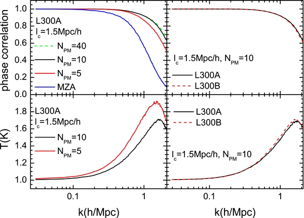
Figure 1. Upper left panel: the phase correlations between N-body simulated density field (L300A) and various modeled density fields as indicated in the panel. Here NPM is the number of steps adopted in a PM model and lc is the grid cell size. Upper right panel: the phase correlations between the simulated density fields and the corresponding PM density fields with NPM = 10. Lower left panel: the density transfer functions for PM models with NPM = 5 and 10. Lower right panel: density transfer functions for PM model with NPM = 10, derived from two simulations. The grid cell size is set to 1.5 h−1 Mpc for all cases.
In order to further characterize the phase correlation, we introduce a quantity, k95, which is defined to be the wavenumber at which the correlation coefficient defined in Equation (33) decreases to 0.95. A larger k95 therefore indicates a more accurate model prediction. We show k95 as a function of NPM for various lc in the left panel of Figure 2. For all the cell sizes examined, k95 first increases with NPM, and then remains at an almost constant level. For a given grid cell size lc, there is thus an upper limit in the performance of the PM model, which is consistent with the results shown in Figure 1. Of course, the level of the best performance increases as lc decreases. For instance, the value of k95 for lc = 3, 1.5, and 0.75 h−1 Mpc is about 0.38, 0.80, and 1.78 h Mpc−1, respectively (see the upper right panel of Figure 2), and is roughly proportional to 1/lc. Moreover, these results suggest that, for a given lc, there is a minimum NPM such that the performance of the PM model almost reaches its best and any further increase in NPM no longer makes significant improvement. This minimum NPM roughly scales as $1/l_{\rm c}^{2}$, as shown in the lower right panel of Figure 2, and is about 3, 10, and 40 for lc = 3, 1.5, and 0.75 h−1 Mpc, respectively.
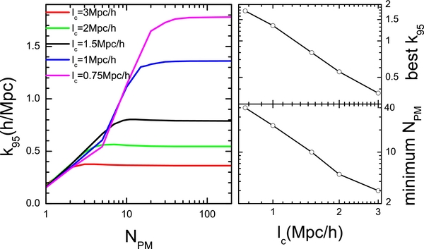
Figure 2. Left panel: the parameter k95 as a function of NPM for different grid cell sizes, lc, as indicated in the figure. Here k95 measures the scale at which the phase correlation between the PM density field and the original simulated density field is 0.95. Right panels: the best k95 and the required minimum NPM as a function of lc. All the results are based on the simulation L300A.
For given NPM and lc, significant bias can exist in the PM density field relative to the real density field. In order to correct for this effect, following TZ12, we introduce a density transfer function, T(k), which is obtained by cross-correlating the original simulation and the PM density field (Equation (27)). Note that introducing T(k) into the calculation of the final density field does not change the phase correlation shown above. As an example, the lower left panel of Figure 1 shows the transfer function for lc = 1.5 h−1 Mpc and NPM = 5 or 10. As expected, T(k) is almost unity at large scales and increases gradually with increasing k until k ∼ 1.5 h Mpc−1. A downturn is observed in the transfer functions at small scales, indicating a rapid decline in the correlation between the two density fields at such scales. Since the PM model with NPM = 10 (referred to as PM10) is more accurate than PM5, the transfer function for the PM10 model is closer to unity than that for the PM5 model. Similar to the phase correlations, the transfer functions are insensitive to sample variance (see the lower right panel of Figure 1). In what follows, PM model really refers to the PM model combined with the corresponding transfer function.
The other way to reduce the bias produced by the inaccuracy of the PM model at small scales is to smooth both the PM density field and the input density field at small scales before using them to calculate the likelihood function in the HMC. Here we investigate which smoothing scale, Rs, is suitable for our purpose. To this end, we calculate the two point correlation functions for both the PM density field (ξPM) and the original, simulated density field (ξSIM), both smoothed with the same smoothing scale. Figure 3 shows the ratio, ξPM/ξSIM, for a number of smoothing scales. The results are shown for three PM models, one with lc = 1.5 h−1 Mpc and NPM = 10, another with lc = 1 h−1 Mpc and NPM = 20, and the third with lc = 0.75 h−1 Mpc and NPM = 40 (hereafter referred to as PM40). We note again that all the density fields are corrected with density transfer functions. The model predictions are in good agreement with the original ones at large scales for all models, independent of the smoothing scale adopted. At small scales, however, the PM density fields are less clustered than the simulated ones. This discrepancy is significant only when the smoothing scale, in units of lc, is chosen to be too small, but almost vanishes for Rs ⩾ 2lc. This basically says that the PM density field is inaccurate on scales below a couple of grid cells and the difference between the model prediction and the input field on such scales should be suppressed with smoothing. However, choosing a too large Rs will cause a loss of information on small scales. As a compromise we use Rs = 3lc as our fiducial value.

Figure 3. Ratios between the two-point correlation functions measured from the PM and the simulated density fields for three PM models as indicated in the panels. The density fields are smoothed with various smoothing scales, Rs, as indicated.
4. APPLICATIONS AND TESTS OF THE HMC+PM METHOD
4.1. Setting Parameters for the HMC
Before describing the applications of our PM based HMC (HMC+PM), we briefly describe how to specify the parameters in the HMC and the PM model. We divide the simulation boxes into $N^3_{\rm c}$ grid cells and use a Gaussian kernel with a smoothing scale of Rs to smooth the particle distributions at redshift zero on to the grids. The resultant density fields, denoted by ρsi(z = 0), are what we want to match in the reconstructions [i.e., ρinp = ρsi(z = 0)].
Our dynamic model consists of two parts. First, the Zel’dovich approximation has one parameter, the initial redshift zi. In this paper we set zi = 36, which is the same as that for the initial conditions of the L300 simulations. Second, the PM model (including the transfer function) has two parameters, the grid cell size, lc, and the number of time steps, NPM. The computation time for a PM model is proportional to NPM and $1/l^3_{\rm c}$. As a compromise between computation time and model precision, we adopt two PM models— PM10 with lc = 1.5 h−1 Mpc and NPM = 10, which is implemented in the reconstructions of the L300 series; and PM40 with lc = 0.75 h−1 Mpc and NPM = 40, used in the reconstructions of the L100 series. The corresponding Nc is 200 for L300 and 134 for L100.
According to the tests shown here, we choose the smoothing scale Rs = 3lc in our HMC runs to make sure that the bias in the PM density field on small scales is sufficiently suppressed. A series of tests were performed in W13 to tune other HMC parameters. Following their results, we adopt nmax = 13, τmax ≈ 0.1 and set σinp(x) = μρsi(x) with μ = 0.5. The weight field w(x) is set to be unity for all grid cells.
4.2. Applications to Simulated Density Fields
We use the four N-body simulations—L300A, L300B, L100A, and L100B—to test our HMC+PM method. Note again that PM10 and PM40 are adopted for the reconstructions of the L300 and L100 series, respectively. The input density field ρinp = ρsi(z = 0) is smoothed with a smoothing scale Rs = nslc, and ns are set to be 3 and 4 for L300 and L100, respectively. The initial set of δ(k) is randomly drawn from the prior Gaussian distribution, G(δ(k)), as shown in Equation (1). The Hamiltonian masses are computed twice during the entire process. The first time is at the beginning. After proceeding 50 or 80 accepted chain steps, the mass variables are updated once with the current Hamiltonian forces and retained all the way to the end. Computations are made for 2000 (3000) HMC steps for the L300 (L100) series, and the acceptance rates for the reconstructions of the L300 and L100 series are about 83% and 96%, respectively. The left and middle panels of Figure 4 show $\chi ^2_{w}\equiv \chi ^2/\sum _{\bf x}w({\bf x})$ as a function of the chain step. The value of $\chi ^2_w$ drops sharply at the beginning (the burn-in phase), and then remains almost constant after about 500 to 1000 chain steps (the convergence phase). The $\chi ^2_w$ values of the converged steps are about 0.004 (L300) and 0.002 (L100), showing that the predicted density fields after convergence match the input ones well.

Figure 4. $\chi ^2_{w}=\chi ^2/\sum _{\bf x}w({\bf x})$ as a function of chain step for four HMC reconstructions. The left panel shows the results for the L300 series, while the middle and right panels show the results for the first and second HMC parts for the L100 series. The first HMC part adopts a larger smoothing scale than the second part.
For the reconstruction of the L100 series, a further HMC process is carried out to increase the reconstruction accuracy. This time the input density field is still ρsi, but is smoothed with a smaller smoothing scale, Rs = 3lc = 2.25 h−1 Mpc. The initial set of δ(k) is not randomly generated, but taken from the linear density field output at the 2700th step of the first HMC process, and so are the Hamiltonian masses. The new fictitious systems are then evolved for an additional 2000 steps, and the acceptance rates are about 95%. The right panel of Figure 4 shows $\chi ^2_{w}$ as a function of chain step for the additional runs. At the first step, $\chi ^2_{w}$ is about 0.02, which is much larger than the final one of the first HMC run. It is ascribed to the smaller smoothing scale adopted here. One can see that two-phase behavior is also conspicuous. After a quick decline within the first 200 steps, $\chi ^2_w$ converges to about 0.004. Because the initial set of δ(k) is not random, the decrease in the amplitude of $\chi ^2_{w}$ in the second part of the HMC is much slower. We note that the two-phase behavior is commonly seen in HMC runs (e.g., Hanson 2001; Taylor et al. 2008). As discussed in W13, the fictitious system in question actually mimics a cooling system in a gravitational potential well. The reset of momenta at the beginning of every chain step (see Section 2.1) is an analog to the cooling process, which makes the system fall continuously and eventually reach the bottom region of the potential well (i.e., around the posterior peak we are searching for).
On the scale of 4.5 h−1 Mpc (2.25 h−1 Mpc), the RMS (root mean square) difference between ρinp and ρmod is about $\mu \sqrt{2\chi ^2_w}\simeq 4.5%$ (4.6%) for the L300 (L100) series. This is an accurate match, indicating that the second constraint in our reconstruction, namely that ρmod matches ρinp, is well satisfied. In order to check whether our reconstruction also meets the first constraint (i.e., the prior Gaussian distribution with a given linear power spectrum), we show in Figure 5 the power spectra measured from the reconstructed linear density fields at the final chain steps, with the original linear spectra overplotted for comparison. Over the entire range of wavenumbers, the reconstructed initial spectra are in good agreement with the original. However, upon closer examination we see some small deviations. For example, the reconstructed linear spectra contain a small bump (less than 10%) at the intermediate scale (k ∼ 0.9 h Mpc−1 in the L100 series). A similar but significantly stronger bump is also seen in the reconstructed linear spectra of W13, Kitaura (2013, their Figure 2) and Ata et al. (2014).
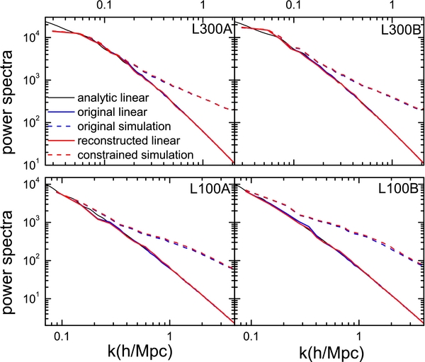
Figure 5. Blue and red solid lines show the original and reconstructed linear power spectra. The blue and red dashed lines show the z = 0 power spectra measured from the original input simulations and corresponding CSs. The black solid lines show the analytic linear power spectrum.
In order to understand the origin of this discrepancy, we apply our HMC+PM reconstruction with PM density fields as input. Since the input field is generated with the same PM model as that used in the HMC, no bias is expected from the inaccuracy of the PM model. As shown in Appendix C, even in such cases there is still deviation on scales ∼Rs, below which the prior term of the Hamiltonian force starts to dominate over the likelihood term. Fortunately, the deviation is quite small (typically less than 10%) and can be moved to small scales of no practical importance by adopting a sufficiently small lc (so that Rs is sufficiently small).
For a random Gaussian field, $d_{{\rm n},j}({\bf k})\equiv \delta j({\bf k})/\sqrt{P{\rm lin}(k)/2}$ should obey a Gaussian distribution with σ = 1, independent of the wavenumber k. Figure 6 shows the distributions of dn, j(k) for three different wavenumbers, together with a Gaussian function with σ = 1. These distributions match the Gaussian distribution very well, even in the large |dn, j(k)| tails. The fluctuations at the tails are due to small number statistics. We have also calculated the third- and fourth-order moments of the distributions, and estimated the corresponding skew and kurtosis (using Equations (6.43) and (6.44) in Mo et al. 2010). Both are found to be very close to zero. This demonstrates that our reconstruction recovers the Gaussianity of the linear density field very well.
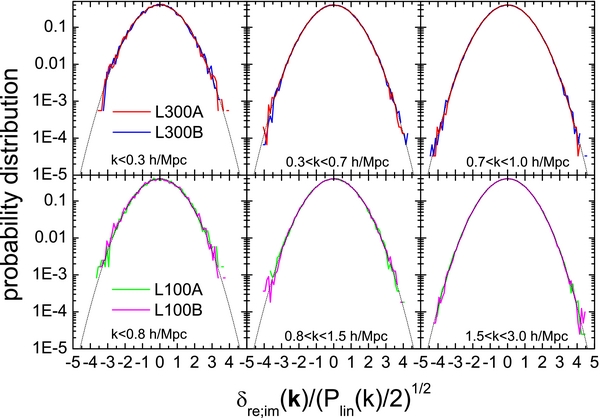
Figure 6. Distributions of $\delta {j}({\bf k})/\sqrt{P{\rm lin}(k)/2}$ at three different scales as indicated in the panels. Here δ(k) is the reconstructed linear density field. The smooth curves are Gaussian distributions with dispersion σ = 1.
At small scales the Hamiltonian forces are dominated by the prior term, as the likelihood term is strongly suppressed by the smoothing (see Appendix C). Consequently the phases of the reconstructed δ(k) are expected to be random on small scales. To quantify on which scales the reconstructed δ(k) matches the original ones well, we measure the phase correlation between the two linear density fields. The results are shown as solid lines in the two left panels of Figure 7. For the L300 series, the correlation coefficients are larger than 0.95 at k < 0.28 h Mpc−1, and decline gradually to 0.5 at k ∼ 0.47 h Mpc−1. For the L100 series the phase correlation is even better, with the correlation coefficient reaching 0.95 at k ∼ 0.36 h Mpc−1 and declining to 0.5 at k ∼ 0.85 h Mpc−1. The correlation is still significant (Cp ∼ 0.1) at k ∼ 1.3 h Mpc−1. The improvement is clearly due to the better PM model, which can better recover the phase information on small scales. Note that the results of the two reconstructions in the same series are very similar, again demonstrating the robustness of our HMC+PM method.
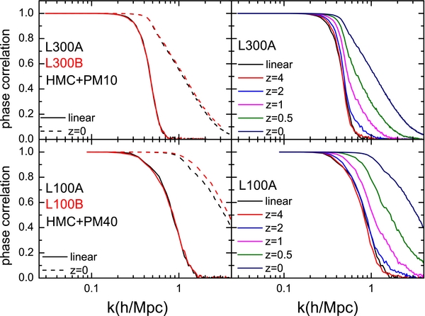
Figure 7. Left panels: the solid lines are the phase correlations between the original and reconstructed linear density fields, while the dashed lines are the phase correlations between the original (input) simulations and the corresponding CSs at redshift zero. Right panels: the phase correlations between the original simulation and the CS at various redshifts. The black line is the correlation of the linear density fields.
So far, we have shown the results of the linear density field obtained from the final chain step of each reconstruction. We also checked the results at other steps after burn-in and found that they have almost the same statistical properties as the final chain step. Because our goal is to reconstruct δ(k) rather than draw a posterior ensemble of linear density fields, we will not present the results for chain steps other than the final one.
5. N-BODY SIMULATIONS OF THE RECONSTRUCTED INITIAL DENSITY FIELDS
To further investigate the accuracy of our method, we use the reconstructed linear density fields to set up initial conditions and evolve them to the present day with the N-body code Gadget-2 (Springel 2005). These new simulations are referred to as CS. The initial conditions are sampled with the same number of N-body particles as in the corresponding original simulations. The Nyquist frequency for these initial conditions is larger than krc = Ncπ/L, which is the largest working frequency of our HMC method. We complement the Fourier modes at k > krc by sampling δ(k) from the prior Gaussian distribution, G(δ(k)). In the following a suffix “-CS” is added after the name of an original simulation to denote the corresponding CS. For example, L100A-CS denotes the CS of L100A. The corresponding density field of a CS is denoted by ρcs.
The CS power spectra at redshift zero are presented in Figure 5. As can be expected from the good accuracy in the reconstructed linear density fields, the CS power spectra match their original counterparts well. The phase correlations between ρcs and ρsi at z = 0 are shown as dashed lines in the left two panels of Figure 7. The correlations are very tight. For example, the L100-CSs almost perfectly match the original ones all the way to nonlinear scales, k ∼ 1.0 h Mpc−1. Even at highly nonlinear scales (k ∼ 3.4 h Mpc−1), about half of the phase information is recovered. The correlations are much stronger than that obtained from the HMC+MZA method. The latter predicts a more rapid decrease of the correlation function with increasing k, reaching 0.5 at k ∼ 1 h Mpc−1 (W13). The improvement of our HMC+PM over the HMC+MZA is clearly due the more accurate PM model used in the HMC+PM for evolving the cosmic density field. The phase correlation between ρcs and ρsi is also much tighter than that of the corresponding linear density fields (solid lines). For instance, at k = 1 h Mpc−1 the correlation between the linear density fields is only modest for the L100 series, in contrast to the almost perfect correlation between the fully evolved density fields (dashed lines). This phenomenon can be readily interpreted by nonlinear mode coupling, in which the small-scale power of a nonlinear density field is partly produced by the large-scale power (e.g., Tassev & Zaldarriaga 2012a). Thus, even phase correlation is absent on small scales between the reconstructed and original linear fields; it can be generated by the phase correlation on large scales that are present in the linear fields.
Since the nonlinear effect is more important at lower redshift, the mode coupling effect is expected to be less significant at high z. To demonstrate this, we show the phase correlations between ρcs and ρsi at five different redshifts, together with that for the initial density fields, in the right panels of Figure 7. Take the results for L300A as an example (the upper right panel). The correlation at z = 4 is very similar to that of the linear field, indicating that mode coupling has not taken its effect. At z = 2, the correlation coefficient is enhanced significantly at k ∼ 0.9 h Mpc−1, but remains unchanged at k ∼ 0.5 h Mpc−1. As the evolution proceeds to z = 0.5, the effect becomes visible over the entire range of wavenumbers, where the initial phases are not well constrained. Similar behavior is also found for L100A, as shown in the lower right panel. This demonstrates again that an accurate dynamic model of structure evolution is required in order to have accurate reconstruction in the nonlinear regime.
In Figures 8 and 9, we compare mass densities in the CSs with those in the input simulations at four different redshifts. The density fields are smoothed within Gaussian windows with radii the same as Rs adopted in the corresponding HMC runs (i.e., 4.5 h−1 Mpc for L300, and 2.25 h−1 Mpc for L100). The three contours in each panel encompass 67%, 95%, and 99% of the grid cells in the whole simulation box. The densities of the CS in individual cells are tightly and linearly correlated with the original ones over a large dynamic range; for L100 this correlation extends from $\rho /{\bar{\rho }}= 0.1$ to about 50 at redshift zero. The CS do not show any significant bias, and at z = 0 the typical dispersion in the ρsi–ρcs relation is about 0.05 dex for both L300 and L100. Interestingly, the typical dispersion does not depend significantly on redshift; the seemingly looser relations at higher z are due to the smaller ranges in density. However at high z the dispersion is larger for higher densities, because small-scale modes are not well constrained in the initial conditions and mode coupling has not fully developed at high z.
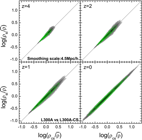
Figure 8. Density–density plots between the original simulation, L300A, and the corresponding CS at various redshifts. The density fields are smoothed with a Gaussian of radius 3 h−1 Mpc. The three contours encompass 67%, 95%, and 99% of all the grid cells in the simulation box. All these densities are scaled with $\bar{\rho }$, which is the mean density of the universe at the redshift in question.
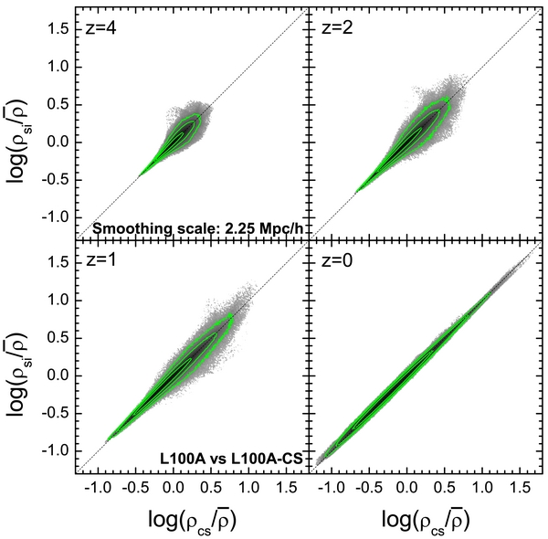
Figure 9. Same as Figure 8 but for the L100A and its CS filtered with a Gaussian function of smaller radius 2.25 h−1 Mpc.
Figure 10 shows some renderings of the three-dimensional (3D) density fields of L100A (left) and L100A-CS (right) at four different redshifts. Particles are color-coded by local densities calculated using the Delaunay density estimator developed by Schaap & van de Weygaert (2000), with white clumps corresponding to massive halos. The two maps look very similar at z = 0. Almost all large structures in the original simulation, such as massive clusters, filaments, and underdense voids, and even some small details, are well reproduced. In particular, the CS accurately recovers the topological structures of the cosmic web, suggesting that the large-scale environment of dark matter halos, which is an important factor affecting halo formation (see, e.g., Wang et al. 2011), is well reproduced. At higher z, the similarity is also remarkable, in particular on large scales. On small scales, there are noticeable differences that become more significant with increasing redshift, which is consistent with the phase correlation results shown in Figure 7. These comparisons demonstrate that our method can recover the formation history of the large-scale structure with high accuracy.
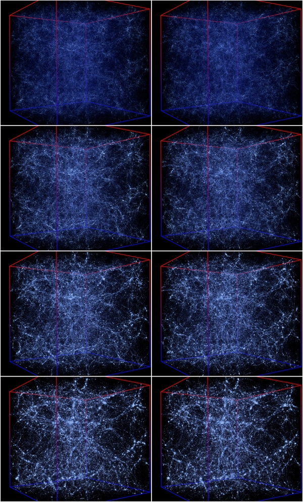
Figure 10. 3D renderings of the particle distributions, color-coded by density, in a cubic 100 h−1 Mpc box. The left panels show the particles in the simulation L100A and the right panels show those in the corresponding L100A-CS. The panels (from top to bottom) show the results at z = 4, 2, 1, and 0, respectively.
Halos are the key components in the build-up of structure in current CDM cosmogony and are thought to be the hosts of galaxies. Therefore, a proper reconstruction of halo properties is essential for our future study of galaxies and their relation with the large-scale environment. In a forthcoming paper, we will compare in detail the internal properties, environment and assembly histories of halos and other structures between the input simulations and CSs. Here we only focus on the halo mass function n(Mh) = dn/dlog Mh. We identify halos using the standard friends-of-friends (FOF) algorithm (Davis et al. 1985) with a link length that is 0.2 times the mean inter-particle separation. Following Warren et al. (2006), we calculate the mass of a halo as $M_{\rm h}=m_{\rm p}N_{\rm h}(1-N_{\rm h}^{-0.6})$, where mp is the particle mass and Nh is the total particle number in a halo. This mass definition is used to correct for some statistical effects of using only a finite number of particles to estimate the mass of a FOF halo.
The halo mass functions at various redshifts obtained from L300A-CS and L100A-CS are shown in Figures 11 and 12, with the error-bars representing Poisson fluctuations in individual mass bins. These CS mass functions are well matched by both the theoretical prediction (Sheth et al. 2001) and those obtained from the corresponding original simulations. To inspect the results in more detail, we show in Figure 13 the ratio of the halo mass function between the CS and the original simulation, ncs(Mh)/nsi(Mh). If nsi(Mh) = 0 in a mass bin, it is replaced by the corresponding value of the theoretical halo mass function. In order to reduce the fluctuations at the high mass end, halos are re-binned into fewer mass bins. As one can see, although the halo mass functions of the reconstructed density fields are in overall good agreement with the original ones, there is very weak but noticeable bias. This bias is not expected, as the initial density field is well reproduced in both power spectrum and Gaussianity. As will be shown later, the reconstruction apparently can introduce a very subtle non-Gaussian effect, which in turn can affect the precision of the predicted halo mass function. This effect becomes more important when a less accurate model of structure evolution is adopted.
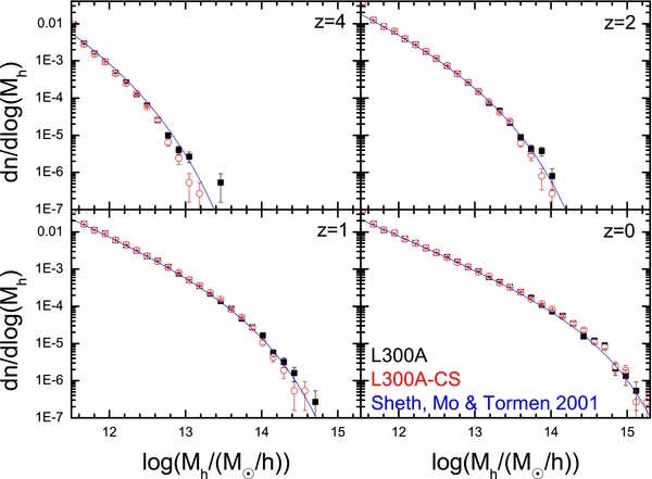
Figure 11. Halo mass functions obtained from L300A (squares) and L300A-CS (red circles) at four different redshifts. The blue lines represent the theoretical predictions (Sheth et al. 2001).
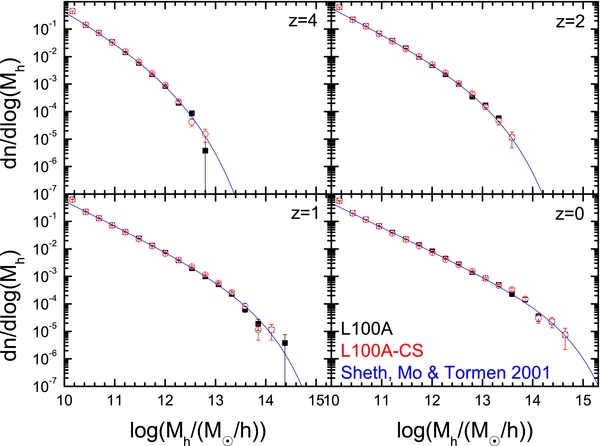
Figure 12. Same as Figure 11 but for L100A and L100A-CS.
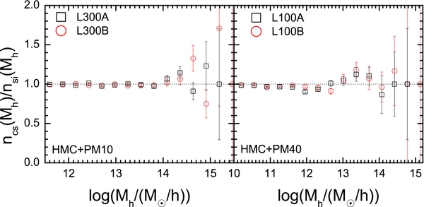
Figure 13. Ratio between the halo mass function obtained from the CS, ncs, and that from the original simulation, nsi.
6. COMPARING RESULTS OBTAINED FROM DIFFERENT MODELS OF STRUCTURE EVOLUTION
A number of different structure evolution models have been adopted in the literature for the reconstruction of the initial cosmic density field. Here we compare the performances of some of them and show that our HMC+PM is superior.
In our earlier paper (W13) we adopted the MZA model, which was developed by TZ12. The phase correlation between the density field reconstructed from the HMC+MAZ method with the input density field is plotted in the upper left panel of Figure 1. For this model, k95 ∼ 0.33 h Mpc−1 and this is very similar to that shown in TZ12 for different cosmological parameters. The phase correlation for 2LPT, which is adopted by Jasche & Wandelt (2013) and Kitaura (2013) to reconstruct the initial density fields from the galaxy density field, has k95 = 0.37 h Mpc−1, as shown in TZ12. More recently, Heß et al. (2013) employed a modification of the 2LPT, the ALPT developed by Kitaura & Heß (2013), in their reconstruction. As shown in Figure 4 of Kitaura & Heß (2013), the ALPT model can achieve k95 ∼ 0.45 h Mpc−1, better than the 2LPT. For our HMC+PM method, Figure 2 shows that the values of k95 achieved by PM5 and PM10 are 0.67 and 0.80 h Mpc−1, respectively, which is much better than all the earlier models. Indeed, our test showed that the performances of the 2LPT and the ALPT are only between our PM models with NPM = 2 and 3. Clearly, the PM model with a modest number of time steps is by far the best model that can be implemented into the HMC method.
For further tests, the linear density field is reconstructed from the L300A simulation using both the HMC+MZA and the HMC+PM5. The density transfer function for PM5 is given in the lower left panel of Figure 1, while that for MZA is adopted from TZ12. Since the HMC runs employing the same model of structure evolution give very similar results (see, e.g., Figure 7), only one run is performed for each model. Similar to the finding in W13, the reconstructed linear power spectra from these two runs match well the original ones, except for a significant bump on intermediate scales. We follow W13 to renormalize the amplitudes of the modes in the bump so that the power spectrum matches the original. As shown in W13, even with the renormalization, the distributions of $d_{{\rm n},j}({\bf k})=\delta j({\bf k})/\sqrt{P {\rm lin}(k)/2}$ are still very close to Gaussian with σ = 1. We use the linear density fields so obtained to set up initial conditions, and follow the evolutions of the density fields with the N-body code described previously.
Figure 14 shows the mass function ratio, ncs(Mh)/nsi(Mh), at z = 0 for the three models: HMC+PM10, HMC+PM5, and HMC+MZA. The halo mass function for the MZA model deviates significantly from the original; it produces too many massive halos at Mh > 1014.3 h−1 M☉ and too few halos of 1013.5 h−1 M☉. Second, there is a clear trend that the mass function in the CS gradually converges with the original as the accuracy of the model increases, from MZA to PM5 to PM10. For PM10, the CS mass function is already quite close to the original. Recently, Heß et al. (2013) found that their CSs of the linear density fields constructed from the ALPT model significantly overproduce massive halos and underproduce small-mass halos relative to the reference mass functions. This is exactly the same as we find here when a model of low accuracy is used to evolve the cosmic density field, although the Bayesian approach they adopted is different from ours. The deviation they found is therefore more likely a result of the inaccuracy of the ALPT, rather than the cosmic variance.
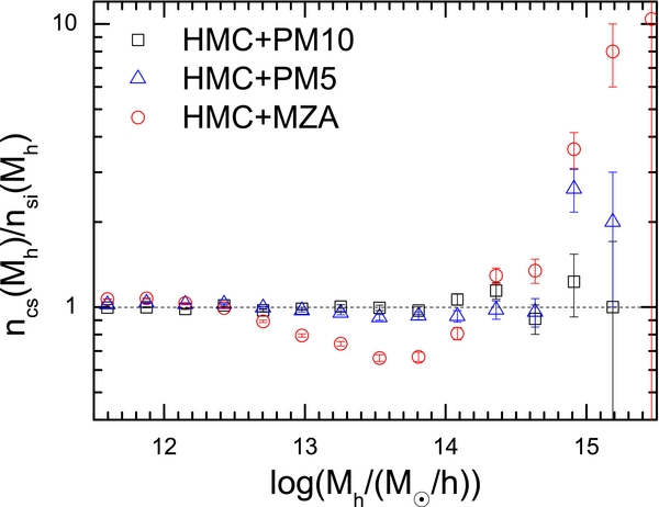
Figure 14. Ratio between the halo mass function derived from the reconstructed final density field and that from the original density field. Results are shown for different models of structure evolution, as indicated in the figure. The results are all based on L300A.
One possible reason for this deviation is that the HMC induces spurious correlations in the reconstructed δ(k) if the model of structure evolution is not sufficiently accurate. Most of the approximations, which cannot properly handle highly nonlinear dynamics on small scales, tend to underestimate the density in high density regions, in particular around halos. Thus the parameter χ2, which the HMC process attempts to minimize, is contributed by two different sources. One is the difference between the reconstructed and the real δ(k), and the other is the underestimation of the power spectra on small scales due to the use of approximate dynamics. During the evolution of the Hamiltonian system, the HMC tries to tune δ(k) to compensate for the lost power in two ways: to enhance the amplitude of δ(k), which is seen in the reconstructed linear power spectra (see W13; Kitaura 2013; Ata et al. 2014), and to introduce some non-Gaussianity into δ(k).
To verify the latter probability, we first derive a smoothed version of the reconstructed linear density field, δ(x, rth), where the smoothing is done with a top-hat kernel with radius rth. We then measure the variance (κ2 ≡ σ2), skewness (κ3), and kurtosis (κ4) of the smoothed field. For a random Gaussian field, it is easy to prove that κl = 0 for all l > 2. Thus any non-zero, high-order κl signifies non-Gaussianity. Figure 15 shows the three quantities as functions of rth for the original linear density field and the reconstructed linear density fields based on PM10, PM5, and MZA. For comparison, we also present the results measured from 19 random Gaussian fields.
Figure 15. Variance (σ2), skew (κ3), and kurtosis (κ4) of the linear density fields in real space as a function of smoothing scale rth (top-hat smoothing kernel). The black dashed lines show the results measured from the original linear density field of L300A. The solid lines show the results measured from the reconstructed linear density fields based on different models of structure evolution, as indicated in the right panel. The gray bands show the spread of 19 linear density fields randomly sampled from the prior Gaussian distribution, G(δ(k)), given in Equation (1).
The three reconstructions exhibit almost identical σ2(rth) as the original, which is expected because σ2(rth) is directly related to the linear power spectrum. However, there are clear differences in κ3 and κ4 between the three reconstructions and the original linear density field. By construction, these two quantities should be close to zero. The reconstructed linear density field based on PM10 exhibits small nonzero κ3 on small scales, but the deviation is still within the gray region that represents the variance among the 19 random Gaussian fields. The situation is very similar for κ4. Thus, no significant signal for non-Gaussianity is present in the reconstructed δ(k) based on PM10. In contrast, the non-Gaussianity is quite significant for PM5, and is the strongest for MZA. Such non-Gaussianity is hard to see in the distribution function of δ(k), but it is the source of bias in the predicted halo mass function. As the densest and most massive objects in the cosmic density field, massive halos are sensitive to the tail of the density distribution. These tests support our hypothesis that the origin of the deviation in halo mass function is non-Gaussianity.
Another potential issue is the smoothing scale Rs adopted for the three tests shown here, all being 3lc = 4.5 h−1 Mpc. According to the results of our two-point correlation function analysis (Section 3.2), this smoothing scale can effectively erase the difference between the model prediction of PM10 and the simulation, and so the result of the halo mass function is not biased by the inaccuracy of the model. For PM5 and MZA, however, Rs = 4.5 h−1 Mpc may be too small to get rid of the difference between the model and the simulation. This again shows that, in order to increase the accuracy of the reconstruction and simultaneously maintain Gaussianity, a highly accurate model of structure evolution is required. For example, the HMC+PM40 model with Rs = 2.25 h−1 Mpc predicts a phase correlation that is significantly tighter than the prediction of the HMC+PM10 model. Consequently the halo mass function obtained is also in better agreement with the original.
7. SUMMARY AND DISCUSSION
Following the spirit of our previous paper (W13, see also Jasche & Wandelt 2013), we have developed a HMC method to reconstruct the linear (initial) density field from a given input nonlinear density field at low redshift. This method allows us to generate the linear density field based on a posterior probability distribution function including both a prior term and a likelihood term. The prior term ensures that the reconstructed linear density field obeys a Gaussian distribution with a given power spectrum. The likelihood is designed to ensure that the evolved density field from the reconstructed linear density field matches the input nonlinear density field. To improve the accuracy of the reconstruction, we combined the HMC with the PM dynamics. The Hamiltonian force is the most important quantity that guides the chain steps, and we worked out how to compute the Hamiltonian force for the PM model.
To optimize the parameters in the PM model, we made a series of tests to investigate how the quality of the PM model predictions depend on the grid cell size, lc, and the number of time steps, NPM. The minimum NPM required for the PM model to approach its best quality roughly scales as $1/l^2_{\rm c}$, and the wavenumber below which the PM model is reliable scales as 1/lc. As a compromise between the accuracy of model prediction and computation time, we made HMC runs with two choices: one with lc = 1.5 h−1 Mpc, and the corresponding minimum number of time steps is NPM = 10; the other has lc = 0.75 h−1 Mpc and the minimum number of time steps is NPM = 40. To increase the accuracy of model prediction we used a density transfer function, which is very easy to obtain. The PM10 model can produce more than 95% of the phase information in the corresponding high-resolution N-body simulation down to a scale corresponding to k = 0.8 h Mpc−1. The PM40 model is much more accurate, recovering more than 95% of the phase information all the way down to a highly nonlinear scale, k = 1.78 h Mpc−1. The discrepancy between the PM prediction and the input field on small scales needs to be suppressed in a HMC run. Based on our two-point correlation function analysis, this can be done with a Gaussian filter with a radius Rs ≈ 3lc.
We used four high-resolution N-body simulations as inputs to test the performance of our HMC+PM method. The Fourier modes of the reconstructed linear density fields obey a Gaussian distribution with a variance that is well matched by the original linear power spectrum. The phase-correlation coefficient between the reconstructed and original linear density fields is close to unity on large scales and declines gradually to 0.5 at k ∼ 0.85 h Mpc−1 and k ∼ 0.47 h Mpc−1 for the HMC+PM40 and HMC+PM10 runs, respectively. The RMS in the difference between the original (input) and modeled density fields are only about 4.6%. A weak discrepancy appears around the scale where the ratio between the likelihood and prior terms of the Hamiltonian force is about one, and is due to the compromise the HMC makes between these two terms.
As additional tests, we compared the original simulations with the corresponding CS that are evolved from the reconstructed linear density fields with a high-resolution N-body code. The density fields in the CS are found to match the original ones over a large dynamic range at various redshifts. The typical dispersions in the density–density relation are about 0.05 dex on the scale of 3lc, almost independent of redshift. Visual inspection of the particle distributions also shows that the CSs can reproduce the large-scale structures and their evolution histories. For the HMC+PM40 (HMC+PM10) run, the phase correlation between the CS and the original simulation is very close to unity down to a scale corresponding to k = 1.1 h Mpc−1 (0.5 h Mpc−1), and remains larger than 0.5 all the way to the highly nonlinear regime k ∼ 3.4 h Mpc−1 (1.1 h Mpc−1). In addition, the halo mass functions derived from the CSs match well those derived from the original simulations. The tests based on the four different simulations give very similar results, demonstrating the robustness of our method.
We also investigated how the performance of the HMC method depends on the accuracy of the dynamical model of structure evolution adopted. For a given Rs, a low-quality dynamical model results in a large deviation in the halo mass function, and produces significant non-Gaussianity in the reconstructed linear density field. These results demonstrate the importance of adopting accurate dynamics in the HMC approach of reconstruction, and our HMC+PM method provides such a scheme. The method can achieve very high accuracy as long as the available computational resources allow the implementation of a PM model with sufficiently small lc and sufficiently large NPM.
In the future, we will apply our HMC+PM method to generate the initial conditions for the structure formation in the local universe using observational data. Since our method needs an input density field, the method developed by Wang et al. (2009) will be adopted to reconstruct the present day density field from the SDSS DR7 galaxy group catalog constructed by Yang et al. (2007). This halo-based reconstruction method has been tested in great detail in Wang et al. (2009, 2012, 2013) and has been applied to SDSS DR4 by Muñoz-Cuartas et al. (2011) and to SDSS DR7 by W13. Our HMC+PM method can also be applied to the z ∼ 2 density field reconstructed from the Lyα forest data (Pichon et al. 2001; Caucci et al. 2008). The test based on mock spectra by Lee et al. (2014) suggested that the spatial resolution in such reconstruction can reach a scale of ∼2 h−1 Mpc (in comoving units) at z ∼ 2, which can be handled very easily with our method. These studies showed that there are significant uncertainties in the reconstructed density fields at a given redshift, which may eventually be the main source of uncertainties in future applications. We will come back to this in a forthcoming paper.
The reconstructed initial conditions can be used to run CSs with both dark matter and gas components. This offers a unique opportunity to investigate the formation and evolution of the galaxy population we directly observe. For example, we can model galaxy formation using halos extracted from the CSs combined with semi-analytical models of galaxy formation, or carry out gas simulations directly from the reconstructed linear density field. The comparison between the modeled galaxy population and the observed one is then conditioned on the same large-scale environments, and so the effect of cosmic variance is eliminated or reduced. Furthermore, the predicted distribution and state of the gas component can also be compared directly with observations of the Sunyaev–Zel’dovich effect, X-ray emission, and quasar absorption line systems, to provide a more complete picture of the interaction between dark matter, gas, and galaxies.
We thank Yu Yu for useful suggestion and Kun Cheng for rendering the figures. This work is supported by the Strategic Priority Research Program “The Emergence of Cosmological Structures” of the Chinese Academy of Sciences, grant No. XDB09010400, NSFC (11073017, 11233005, 11320101002, 11121062, 11033006, 11473053, U1331201), NCET-11-0879. H.J.M. would like to acknowledge the support of NSF AST-1109354 and the CAS/SAFEA International Partnership Program for Creative Research Teams (KJCX2-YW-T23). This work made use of the High Performance Computing Resource in the Core Facility for Advanced Research Computing at the Shanghai Astronomy Observatory.
APPENDIX A: ABBREVIATIONS, TERMS, AND QUANTITIES
-
PM model: particle-mesh model;
-
lc: the mesh cell size in a PM model;
-
NPM: number of time steps in a PM model;
-
PMNPM: a PM model with NPM time steps;
-
PMNPM density field: the density field predicted by the corresponding PM model;
-
Modeled density field: the density field predicted by a dynamical model of structure evolution;
-
MZA: modified Zel’dovich approximation;
-
HMC: Hamiltonian Markov Chain Monte Carlo;
-
HMC+PMNPM: a HMC run using a specific PM model;
-
HMC+MZA: a HMC run using MZA;
-
Input density field or ρinp: the density field used to constrain a reconstruction;
-
Original quantities: quantities measured from or related to an input simulation;
-
Rs: the radius of the Gaussian kernel used to smooth both the input density field and the modeled density fields in a HMC run;
-
Reconstructed linear density field: the linear density field reconstructed from an input density field;
-
Reconstructed linear power spectrum: the linear power spectrum measured from a reconstructed linear density field;
-
CS: constrained simulation, the simulation of a reconstructed linear density field; and
-
CS quantities: quantities measured from a CS.
APPENDIX B: CALCULATIONS OF THE LIKELIHOOD TERM OF HAMILTONIAN FORCE
Here, we provide the details of the Hamiltonian force calculation described in Section 2.3. For conciseness, we use N to replace NPM in this Appendix.
B.1. The χ2 Transformation
Following Equation (13) in W13, we have

where $\rho _{\rm d}({\bf x})=[\rho _{\rm mod}({\bf x})-\rho _{\rm inp}({\bf x})]\omega ({\bf x})/\sigma _{\rm inp}^2( {\bf x})$. Inserting the expression of ρmod given by Equation (28) into the above expression, we have
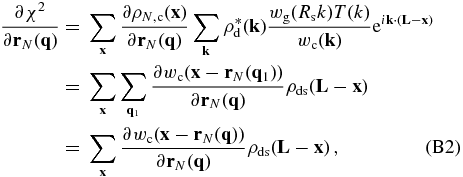
where ρds(x) is the Fourier transformation of $\rho ^{\ast }{\rm d}({\bf k})w{\rm g}(R_{\rm s}k) T(k)/w_{\rm c}({\bf k})$ and L = (L, L, L) so ${\rm e}^{i{\bf k}\cdot \bf L}\equiv 1$. Note that ∂wc(x − rN(q1))/∂rN(q) is nonzero only when ${\bf q}_1=\bf q$. Moreover, ∂wc(x − rN(q))/∂rN(q) is nonzero only in a number of grid cells close to rN(q), which can also be used to speed up the calculation of Equation (B2). Note that χ2 is independent of the final velocity field so that ∂χ2/∂vN − 1/2(q) = 0.
B.2. The Particle-mesh Transformation
Starting from the last step n = N where the derivatives of χ are obtained, we can obtain the derivatives successively at other steps. Suppose we have already obtained ∂χ2/∂rn + 1(q) and ∂χ2/∂vn + 1/2(q). We can use the chain rule to write ∂χ2/∂rn(q) and ∂χ2/∂vn − 1/2(q) as


where the symbol ⊗ stands for matrix multiplication. According to the leapfrog Equations (20) and (21) in the PM model, we have


where $\bf I$ is a unit matrix, and δ(q1 − q) is equal to one when q1 = q, and zero otherwise. In the derivation, we have used the facts that $\partial {\bf r}_{n}({\bf q}1)/\partial {\bf r}{n}({\bf q})=\delta ({\bf q}_1-{\bf q})\bf I$ and ∂rn(q1)/∂vn − 1/2(q) = 0.
Inserting these equations into Equations (B3) and (B4), we obtain


Using Equation (25), the quantity ${\bf F}^{\chi }_{n}({\bf q})$ defined in the second term can be written as
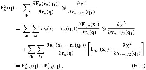
where “·” stands for dot product, and the last line of the equation defines ${\bf F}^{\chi }{n,a}({\bf q})$ and ${\bf F}^{\chi }{n,b}({\bf q})$. The first term of ${\bf F}^{\chi }_{n}({\bf q})$ can be rewritten as
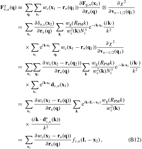
where fv, n(L − x2) is defined by the last line of the equation, and

Thus, dv, n(x1) is equivalent to CIC assignments of “particles” located at rn(q1) with “masses” given by ∂χ2/∂vn − 1/2( q1) to grid points. Its Fourier transform, dv, n(k), can be obtained readily. Since ∂wc(x2 − rn(q))/∂rn(q) is nonzero only at a small number of grid cells close to rn(q), the calculation implied by the last line of Equation (B12) is not time-consuming. The second term of ${\bf F}^{\chi }_{n}({\bf q})$ can be rewritten as

The above transformation can be carried out until n = 0 to give ∂χ2/∂ri(q) = ∂χ2/∂r0(q) and ∂χ2/∂vi(q) = ∂χ2/∂v0(q).
B.3. The Zel’dovich Transformation Finally, the likelihood term of the Hamiltonian force can be written as

Inserting Equations (12) and (13) into the above equation, we have

With the use of the Fourier transform of s(q) given in Equation (14), the Hamiltonian force can be rewritten as,

where Ψ(k1) is the Fourier transform of Ψ(q). Since ∂δ(k1)/∂δj(k) is nonzero only when k1 = ±k, we eventually obtain the expression of the likelihood term of the Hamiltonian force for the real part of δ(k) as

and for the imaginary part as

where Ψre(k) and Ψim(k) are the real and imaginary parts of Ψ(k), respectively.
APPENDIX C: TEST OF THE HMC+PM METHOD USING PM DENSITY FIELDS AS INPUT As shown in Section 4.2, there is always a small bump in the reconstructed linear power spectrum relative to the original. There are two possibilities for this bias. One is the inaccuracy of the adopted dynamical model, and the other is due to the HMC method itself. In order to distinguish these two possibilities, we apply the HMC method to density fields generated by the PM model, so that the first possibility is not an issue and any remaining bias should be due to the HMC method. Two PM density fields in periodic boxes of 300 and 100 h−1 Mpc are used for the test. The density field in the larger box is generated by using PM10, and in the smaller box by using PM40. When applying our method to these PM density fields, the exact same PM models are implemented in the HMC runs. Thus, the PM models adopted in these HMC runs can be regarded as 100 percent accurate.
Four HMC tests are performed. Two are applied to the PM10 density fields smoothed on scales of Rs = 4.5 h−1 Mpc and 3 h−1 Mpc, respectively. The other two use the PM40 density fields smoothed with Rs = 2.25 h−1 Mpc and 1.5 h−1 Mpc as inputs. Figure 16 shows the power spectrum ratio, Prc(k)/Plin(k), where Prc(k) is measured from the reconstructed linear density field and Plin(k) is the original linear power spectrum. In each test, the power spectrum is well recovered on both large and small scales. However, there is a significant but weak (about 10%) dip in the power spectrum ratios. A clear trend is observed—the wavenumber where the dip appears (hereafter kd) increases with decreasing smoothing scale.
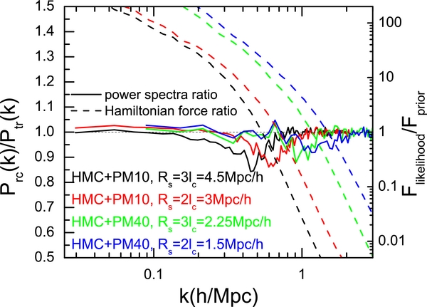
Figure 16. Solid lines show the reconstructed linear power spectra, normalized by the true power spectrum (left axis), Prc/Ptr. The dashed lines show the ratios between the likelihood term and prior term of the Hamiltonian force (right axis). These reconstructions are for PM density fields as input, as detailed in Appendix C.
To understand the origin of this discrepancy, we show in the same figure the average ratio (RF) between the likelihood and prior terms of the Hamiltonian force. This ratio decreases monotonically with increasing k. More importantly, this ratio is about one at the scale kd (see also the discussion in W13). This strongly suggests that the dip in the reconstructed linear power spectrum originates from the competition between the two Hamiltonian force terms. The Hamiltonian force is the most important quantity that drives the evolution of δ(k) in the fictitious system. At large scales where RF ≫ 1, the trajectories of δ(k) are dominated by the likelihood term so they eventually trace well the original linear density field. At small scales where RF ≪ 1, on the other hand, the trajectories of δ(k) are governed by the prior term, so the reconstructed power spectrum matches the original power spectrum, but with totally unconstrained phases. On scales of RF ∼ 1, where the two terms have approximately the same importance, the compromise between them leads to the observed dip. Since the likelihood term increases with the decrease of the smoothing scale, Rs, whereas the prior term does not, it explains why the dip moves toward smaller scales as Rs decreases.
The deviation observed in Section 4.2 also appears around the scale where RF = 1, which is indicative of the same origin. The question is why a bump appears in the applications to N-body simulations, while a dip is found here. This difference is clearly due to the inaccuracy of the PM model relative to the N-body simulation. In general, an approximate model under-predicts the power spectrum at small scales. Although such bias is suppressed by smoothing ( specified by Rs), the reconstructed spectrum is still required to be enhanced by the HMC to compensate for under-prediction by the PM model. The use of a smaller smoothing scale can push the deviation to a smaller scale. Since Rs > 2lc is required (see Section 3.2), a smaller Rs therefore requires a smaller lc and larger NPM.
